Materials+ML Workshop Day 10

Content for today:

• Unsupervised Learning review:

  • Correlation Matrices
  • Dimensionality reduction
  • Principal Components Analysis (PCA)
  • Clustering
  • Distribution Estimation

• Neural networks:

  • Introduction to Neural Networks
  • Neuron Models
  • Activation Functions
  • Training Neural Networks

• Application:

  • Predicting Crystal Structure from the XRD Spectrum

The Workshop Online Book:

https://cburdine.github.io/materials-ml-workshop/

• All Recordings will be made available here after the Workshop

Week 2 Schedule

Session	Date	Content
Day 6	06/16/2025 (2:00-4:00 PM)	Introduction to ML, Supervised Learning
Day 7	06/17/2025 (2:00-4:00 PM)	Advanced Regression Models
Day 8	06/18/2025 (2:00-5:00 PM)	Unsupervised Learning, Neural Networks
Day 9	06/19/2025 (2:00-4:00 PM)	Neural Networks
Day 10	06/20/2025 (2:00-5:00 PM)	Neural Networks, + Advanced Applications

Questions

• Unsupervised Learning review:
  • Feature selection
  • Correlation Matrices
  • Dimensionality reduction
  • Principal Components Analysis (PCA)
  • Clustering
  • Distribution Estimation

Review: Day 8

Unsupervised Learning Models:

• Models applied to unlabeled data with the goal of discovering trends, patterns, extracting features, or finding relationships between data.

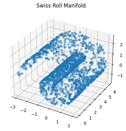
The Importance of Dimensionality

• Dimensionality is an important concept in materials science.
  • The dimensionality of a material affects its properties

• Sometimes, data can be confined to some low-dimensional manifold embedded in a higher-dimensional space.

Example: The "Swiss Roll" manifold

The Correlation Matrix:

• Recall that it is generally a good idea to normalize our data:

$$\mathbf{x} \mapsto \mathbf{z}:\quad z_i = \frac{x_i - \mu_i}{\sigma_i}$$

• The correlation matrix (denoted $\bar{\Sigma}$) is the covariance matrix of the normalized data:

$$ \bar{\Sigma} = \frac{1}{N} \sum_{n=1}^N \mathbf{z}_n\mathbf{z}_n^T $$

Principal Components Analysis (PCA)

• The eigenvectors of the correlation matrix are called principal components.

• The associated eigenvalues describe the proportion of the data variance in the direction of each principal component.

$$\bar{\Sigma} = P D P^{T}$$

• $D$: Diagonal matrix (eigenvalues along diagonal)
• $P$: Principal component matrix (columns are principal components)

Dimension reduction with PCA

We can project our (normalized) data onto the first $n$ principal components to reduce the dimensionality of the data, while still keeping most of the variance:

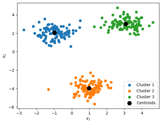
$$\mathbf{z} \mapsto \mathbf{u} = \begin{bmatrix} \mathbf{z}^T\mathbf{p}^{(1)} \\ \mathbf{z}^T\mathbf{p}^{(2)} \\ \vdots \\ \mathbf{z}^T\mathbf{p}^{(n)} \\ \end{bmatrix}$$

K-Means Clustering:

• Identifies the centerpoints for a specified number of clusters $k$

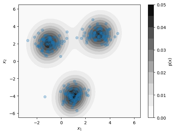
Kernel Density Estimation:

• Estimates the distribution of data as a sum of multivariate normal "bumps" at the position of each datapoint

Today's Content:

Neural Networks

• Introduction to Neural Networks

  • Neuron Models
  • Activation Functions
  • Training Neural Networks

• Application:

  • Training a basic neural network with Pytorch

Neural Networks

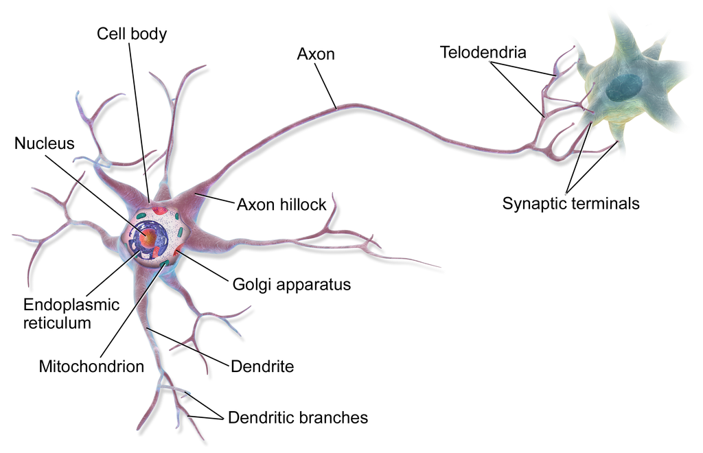
• Neural networks are supervised machine learning models inspired by the functionality of networks of multipolar neurons in the brain:

What can neural networks do?

• They are flexible non-linear models capable of solving many difficult supervised learning problems

• They often work best on large, complex datasets

• This predictive power comes at the cost of model interpretability.

• We know how the model computes predictions, but coming up with a general answer as to why a neural network makes a particular prediction is very hard.

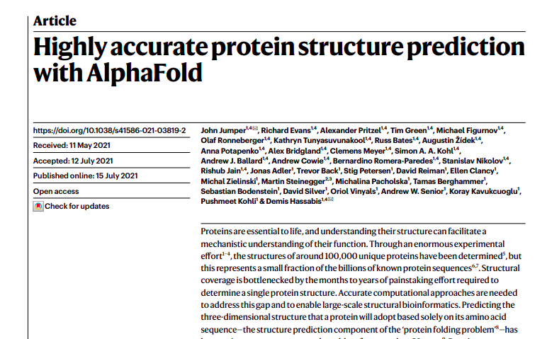
Example: Alphafold (2021)

• The 2024 Nobel prize in chemistry was awarded to Jumper and Hassabis for this work:

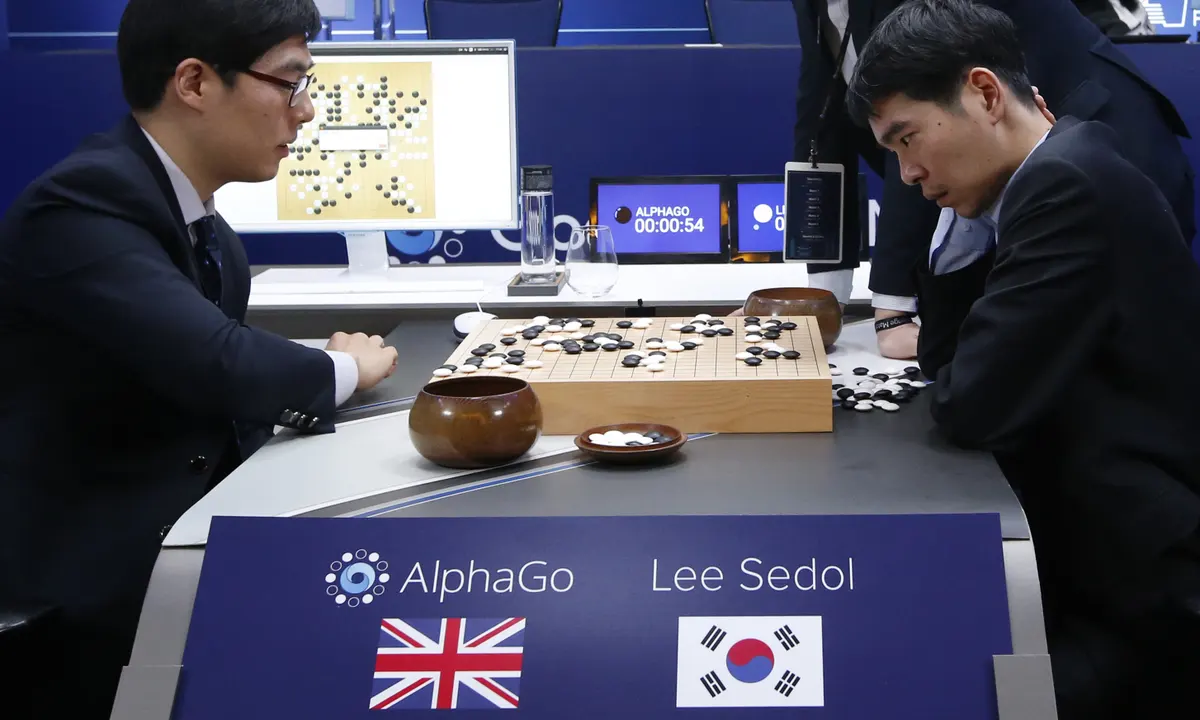
Example: The AlphaGo Model

• A neural network trained entirely through self-play beat international Go champion Lee Seedol.

Standard Feed-Forward Neural Network

• Neural Networks typically consist of individual collections of "neurons" that are stacked into sequential layers:

• Example: Standard "feed-forward" neural network"

A Single Neuron:

• We have alreacy encountered a simple model of a neuron in the form of the Perceptron classifier model:

$$f(\mathbf{x}) = \text{sign}\left( w_0 + \sum_{i=1}^D w_ix_i \right)$$

($\text{sign}(x) = \pm 1$, depending on the sign of $x$)

• $f(x) = +1$ only if a weighted sum of the inputs $x_i$ exceed a given threshold (i.e. $-w_0$)

• This is similar to the electrical response of a neuron to external stimuli

• The Perceptron neuron model has some disadvantages:

  • the function $\text{sign}(x)$ is not continuous and has a derivative of 0 everywhere.

  • It can be difficult to fit this function to data if it is not continuous and differentiable.

The Neuron Activation Function

Instead of the $\text{sign}(x)$ function, we apply a continuous, non-linear function $\sigma(x)$ to the output:

• The function $\sigma(x)$ is called the neuron's activation function.

• The general form of a single neuron can be written as follows:

$$f(\mathbf{x}) = \sigma(\mathbf{w}^T\underline{\mathbf{x}}) = \sigma\left( w_0 + \sum_{i=1}^D w_ix_i \right)$$

• Recall: $$\underline{\mathbf{x}} = \begin{bmatrix} 1 & x_1 & x_2 & \dots & x_D \end{bmatrix}^T$$
• Also: $$\mathbf{w} = \begin{bmatrix} w_0 & w_1 & w_2 & \dots & x_D \end{bmatrix}^T$$

• We can choose different activations $\sigma(x)$, depending on the desired output range of the neuron.

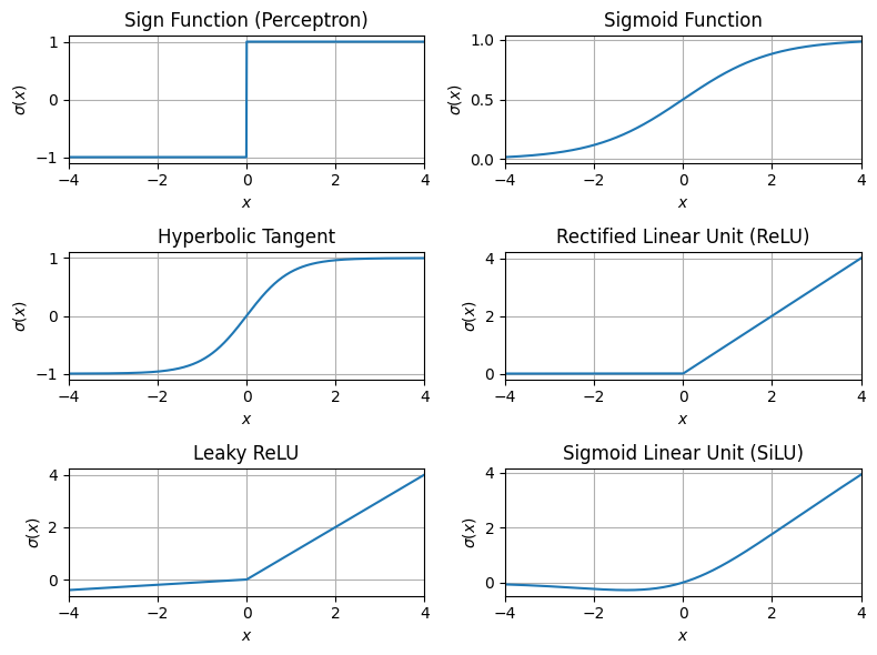
Common Activation Functions:

• Sigmoid function:

$$\sigma(x) = \frac{1}{1 + e^{-x}}$$

• Hyperbolic Tangent:

$$\sigma(x) = \tanh(x) = \frac{e^x - e^{-x}}{e^x + e^{-x}}$$

• Rectified Linear Unit (ReLU):

$$\sigma(x) = \begin{cases} x & x > 0 \\ 0 & x \le 0 \end{cases}$$

• Leaky ReLU:

$$\sigma(x) = \begin{cases} x & x > 0 \\ \alpha x & x \le 0\end{cases}\qquad (0 < \alpha \ll 1)$$

Visualizing Activation Functions

A Layer of Neurons:

• We can combine multiple independent neurons into a layer of neurons.

• The layer computes a vector $\mathbf{a} = f(\mathbf{x})$ of outputs from the neurons:

$$\mathbf{a} = \begin{bmatrix} a_1 \\ a_2 \\ \vdots \\ a_m \end{bmatrix} = f(\mathbf{x}) = \begin{bmatrix} \sigma\left(w_{1,0} + \sum_{i=1}^D w_{1,i}x_i\right) \\ \sigma\left(w_{2,0} + \sum_{i=1}^D w_{2,i}x_i\right) \\ \vdots \\ \sigma\left(w_{m,0} + \sum_{i=1}^D w_{m,i}x_i\right) \end{bmatrix}$$

• Consider a layer of $m$ neurons each with $D+1$ weights.

• We can organize the layer's weights into a matrix $\mathbf{W}$:

$$\mathbf{W} = \begin{bmatrix} w_{10} & w_{11} & \dots & w_{1D} \\ w_{20} & w_{12} & \dots & w_{2D} \\ \vdots & \vdots & \ddots & \vdots \\ w_{m0} & w_{m1} & \dots & w_{mD} \end{bmatrix}$$

• In terms of the weight matrix, we can write the neuron layer function as:

$$\mathbf{a} = f(\mathbf{x}) = \sigma(\mathbf{W}\mathbf{x})$$

A Standard Feed-Forward Neural Network

Training Neural Networks

• We train neural networks through gradient descent with a fixed step size:

$$\mathbf{w}^{(t+1)} = \mathbf{w}^{(t)} + \eta \frac{-\nabla_w \mathcal{E}(f)}{\lVert{-\nabla_w \mathcal{E}(f)}\rVert}$$

• $\eta$ is a constant called the learning rate, and it determines the "step size" of each weight update.

• The numerical process by which $\nabla_w \mathcal{E}(f)$ for layered neural networks is computed is called backpropagation

Gradient Descent

$$\mathbf{w}^{(t+1)} = \mathbf{w}^{(t)} + \eta \frac{-\nabla_w \mathcal{E}(f)}{\lVert{-\nabla_w \mathcal{E}(f)}\rVert}$$

Backpropagation

• As an example, suppose we have two scalar-valued neural network "layers" $g(x)$ and $h(x)$.

• We compose these layers to create a larger model: $$\hat{y} = f(x) = g(h(x))$$

• Computing the gradient of the model loss ($\nabla_w E(f)$) is complicated, but possible given the following:

  • $\frac{\partial E(y, \hat{y})}{\partial \hat{y}}$ (loss function must be differentiable w.r.t. $y$ and $\hat{y}$).
  • $\nabla_w~g(h(x))$
  • $\nabla_w~h(x)$

• In other words, we require each layer to be able to compute the gradient of its weights with respect to the output of the previous layer. We can then apply chain rule to compute the gradients!

• This computation is done most efficiently by working backwards through the neural network layers, using saved outputs of each layer:

$$ \frac{\partial{E}(y, \hat{y})}{\partial \hat{y}}\quad \rightarrow\quad \nabla_w g(h(x)) \quad \rightarrow\quad \nabla_w h(x) \quad\rightarrow\quad ... etc.$$

Neural Network Frameworks

• In Python, there exist many frameworks that can assist you in computing $\nabla_w f(x)$,

  • Pytorch (popular in research settings)
  • Tensorflow (popular in industry settings)
  • JAX (popular for its compatibility with numpy, optimizability)

• These frameworks only require you to define only the "forward" pass of the neural network (e.g. the composition of neural network layers).

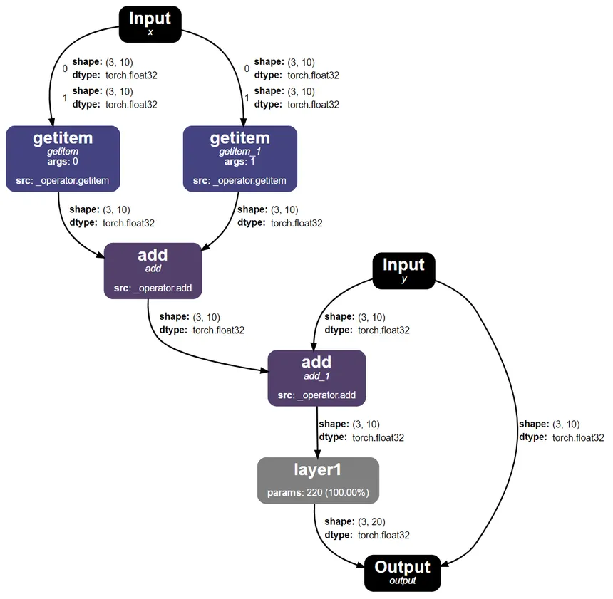
Neural Network Graphs

All of the backpropagation is handled automatically by assembling your neural network layers into a graph.

Introduction to Pytorch

Tutorial: Basic Neural Network in Pytorch

• Goal: Train a neural network to learn the function:

$$f(x_1, x_2) = \frac{\sin(\sqrt{x_1^2 + x_2^2})}{\sqrt{x_1^2 + x_2^2}}$$

Application: XRD Crystal Structure Prediction

• Goal: predict the crystal structure of materials from their X-ray diffraction spectrum.
• We will build and train a neural network in Pytorch.

Questions

Ask me anything about Machine Learning + ML!